


Hey everyone! today I'm going to be talking about rate limiters and different algorithms used to achieve rate limiting, so let's get started!
What is a rate limiter?
A rate limiter puts a limit on the number of requests a server fulfills, it throttles requests that cross a predefined limit, for example, if your service has a rate limit of 500 requests per minute it will block further requests if exceeded that predefined amount.
Rate limiter use cases
Rate limiters can be used in various use cases including the following:
Preventing resource starvation; where sometimes a software error might cause some sort of denial of service attack which is like shooting yourself in the foot and which may cause resource starvation (i.e too many requests and not enough resources to handle them)
Managing policies and quotas; If for example, your API has a free trial amount of calls then you would want to rate limit to that amount.
Controlling data flow; Where it can act as a control valve or regulate the pace of the requests as well as control their distribution among several servers, etc
Avoiding large costs; where rate limiting can prevent having expensive bills, especially when using cloud services.
Algorithms for rate limiting
There are various algorithms for rate limiting, each with advantages and disadvantages;
Token bucket algorithm
Leaking bucket algorithm
Fixed window counter algorithm
Sliding window log algorithm
Sliding window counter algorithm
Token Bucket Algorithm
This algorithm uses the analogy of a bucket with a predefined capacity of tokens, the bucket is continuously being filled with tokens at a constant rate and each time a request comes in, we check if the bucket has an available token, if so we serve the request otherwise rate limiting occurs and we have to wait till the bucket gets filled with a token.
Our parameters consist of:
Bucket capacity; the number of tokens that reside in the bucket
Rate Limit; the number of requests we want to limit per unit of time
Refill rate; which is 1/RLimit and it tells us how often a token gets added to the bucket
Requests count; which is the number of requests flowing in per unit of time
From the above algorithm we can observe the following:
The algorithm can cause a burst in requests if the bucket is filled with tokens that may or may not be beneficial to your business.
Choosing optimal values for a task like this is difficult, it requires careful design and several iterations to reach the optimal values.
The algorithm is space efficient as there are only 4 different parameters that we manipulate
Leaking Bucket Algorithm
This is a variant of the token bucket algorithm but instead of using tokens, it uses a bucket that contains all the incoming requests and processes them at a constant outgoing rate (avoids bursting requests mainly), it uses the analogy of a water bucket leaking at a constant rate where the water represents the requests and leaking is them being processed one after the other in a Queue (First in first out) manner
Our parameters consist of:
Bucket capacity; the maximum capacity of a bucket or the maximum number of requests that can be present in the bucket at a given time
Inflow rate; the rate at which the requests flow into the bucket which may vary and depend on different factors.
Outflow rate; the rate at which the requests get processed
From the above algorithm we can observe the following:
We completely prevent the bursting of request processing due to processing them at a constant outflow rate
Choosing optimal values for a task like this is difficult, it requires careful design and several iterations to reach the optimal values.
A burst of requests can fill the bucket, and if not processed in the specified time, recent requests can take a hit. This may affect the response time of recent requests which might a big problem in our design.
Fixed Window Counter Algorithm
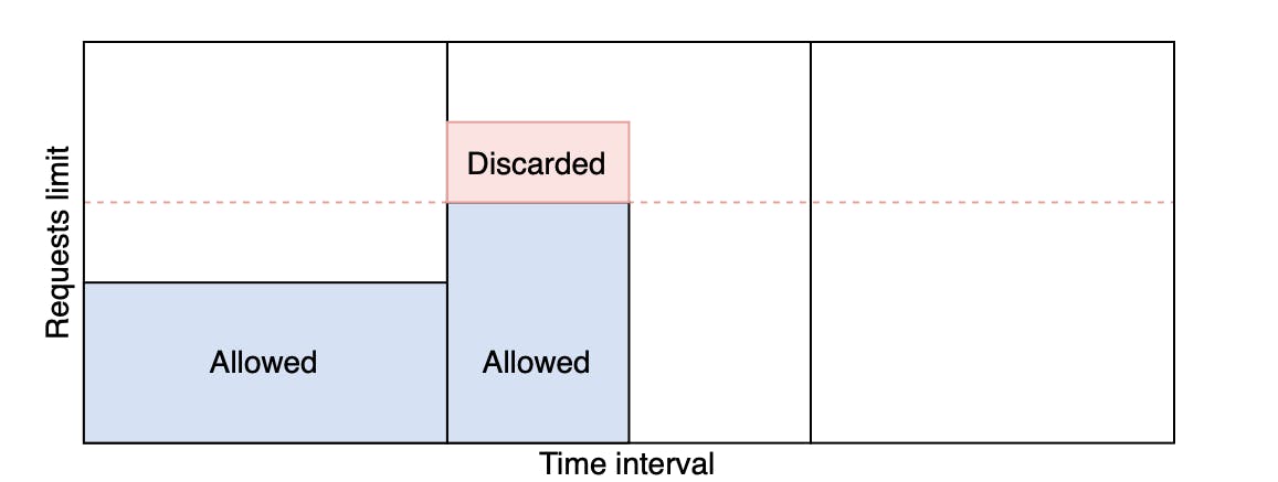
This algorithm divides time into fixed intervals which are called windows and each window has a specific counter that only counts requests belonging to that window, every time a request is made the counter is incremented and requests get dropped when the counter reaches its predefined limit
As seen in the picture below, the dotted line represents the counter limit where requests get discarded after.
There is a significant problem with this algorithm. A burst of traffic greater than the allowed requests can occur at the edges of the window. In the below figure, the system allows a maximum of ten requests per minute. However, the number of requests in the one-minute window from 01:30 to 02:30 is 20, which is greater than the allowed number of requests.
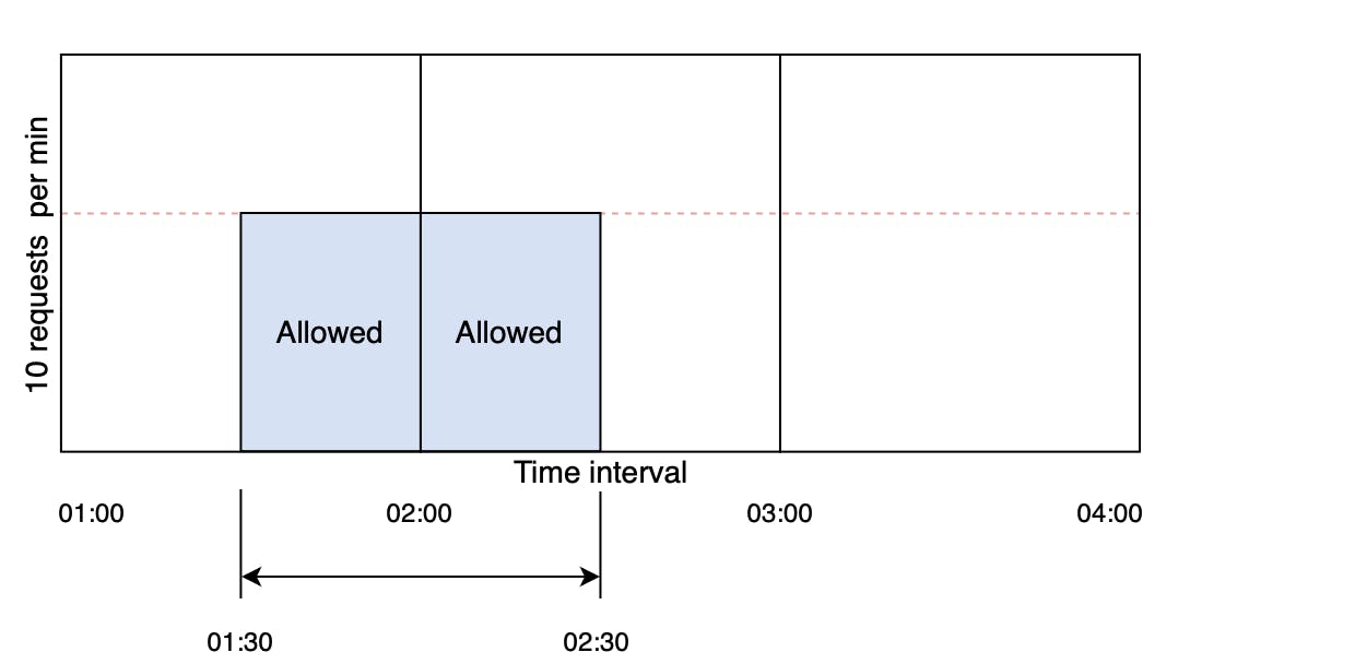
A consistent burst of traffic (twice the number of allowed requests per window) at the window edges could cause a potential decrease in performance.
Our parameters consist of:
Window size; which represents the size of the window which can be in minutes, hours or even days
Rate limit; which represents the number of requests allowed per a time window
Requests count; which is the total number of requests coming in per time window
From the above algorithm we can observe the following:
A consistent burst of traffic (twice the number of allowed requests per window) at the window edges could cause a potential decrease in performance.
It is space efficient due to constraints on the rate of requests.
Sliding window log algorithm
The sliding window log algorithm keeps track of each incoming request. When a request arrives, its arrival time is stored in a hash map, usually known as the log. The logs are sorted based on the time stamps of incoming requests. The requests are allowed depending on the size of the log and arrival time.
The main advantage of this algorithm is that it doesn’t suffer from the edge conditions, as compared to the fixed window counter algorithm.
Let's say a request comes in at 1:00 and the rate is limited to 2 requests per time window, the window will start from 1:00. Another request comes in at 1:45 and it gets served since its less than the limit. Once another one comes in at for example 1:50 it would get rejected as it crossed the rate limit.
After that a request comes in at 2:00, another completely new window starts from here and the same process happens all over again and the old data gets removed from the hashmap.
This approach is more dynamic than the fixed window counter algorithm.
Our parameters consist of:
Log size; which is the number of requests allowed per a specific time frame
Arrival Time; this parameter tracks the incoming requests time stamps' and tracks their count
Time Frame; which is the dynamic time frame that has requests in.
From the above algorithm we can observe the following:
This algorithm doesn't suffer the performance degradation of the fixed window counter due to the window edge problem
It consumes extra memory due to having a hash map and tracking all the requests' timestamps and so on.
Sliding window counter algorithm
Unlike the previously fixed window algorithm, the sliding window counter algorithm doesn’t limit the requests based on fixed time units. This algorithm takes into account both the fixed window counter and sliding window log algorithms to make the flow of requests more smooth. Let’s look at the flow of the algorithm in the below figure.
It gets applied using a mathematical formula that takes into consideration the previous window, the time frame and the overlap which is basically how deep are we into the current time window. I won't go into much depth into this algorithm because things might get complicated but it uses the number of requests basically in the previous time window and the current one in a mathematical formula to calculate a certain value, then this value gets checked against the rate limit of requests (let's say 100 requests per time window) and if it's less than it we can process the request.
Our parameters consist of:
Rate limit; It determines the number of maximum requests allowed per window.
Size of the window; This parameter represents the size of a time window that can be a minute, an hour, or any time slice.
The number of requests in the previous window; determines the total number of requests that have been received in the previous time window.
The number of requests in the current window; represents the number of requests received in the current window.
Overlap time; This parameter shows the overlapping time of the rolling window with the current window.
From the above algorithm we can observe the following:
The algorithm is also space efficient due to limited states: the number of requests in the current window, the number of requests in the previous window, the overlapping percentage, and so on.
It smooths out the bursts of requests and processes them with an approximate average rate based on the previous window.
Summary
There are different algorithms for rate limiting and the key to selecting the right one for you is to answer the question "what do I want to do?". Having an answer to this question will give you a great head start in choosing the algorithm you want to implement.